Diversity and ordination analysis
Xiaotao Shen xiaotao.shen@outlook.com
2026-03-04
Source:vignettes/relative_intensity.Rmd
relative_intensity.RmdThis article introduces the lightweight analysis layer built on top
of microbiome_dataset.
library(microbiomedataset)
data("global_patterns", package = "microbiomedataset")
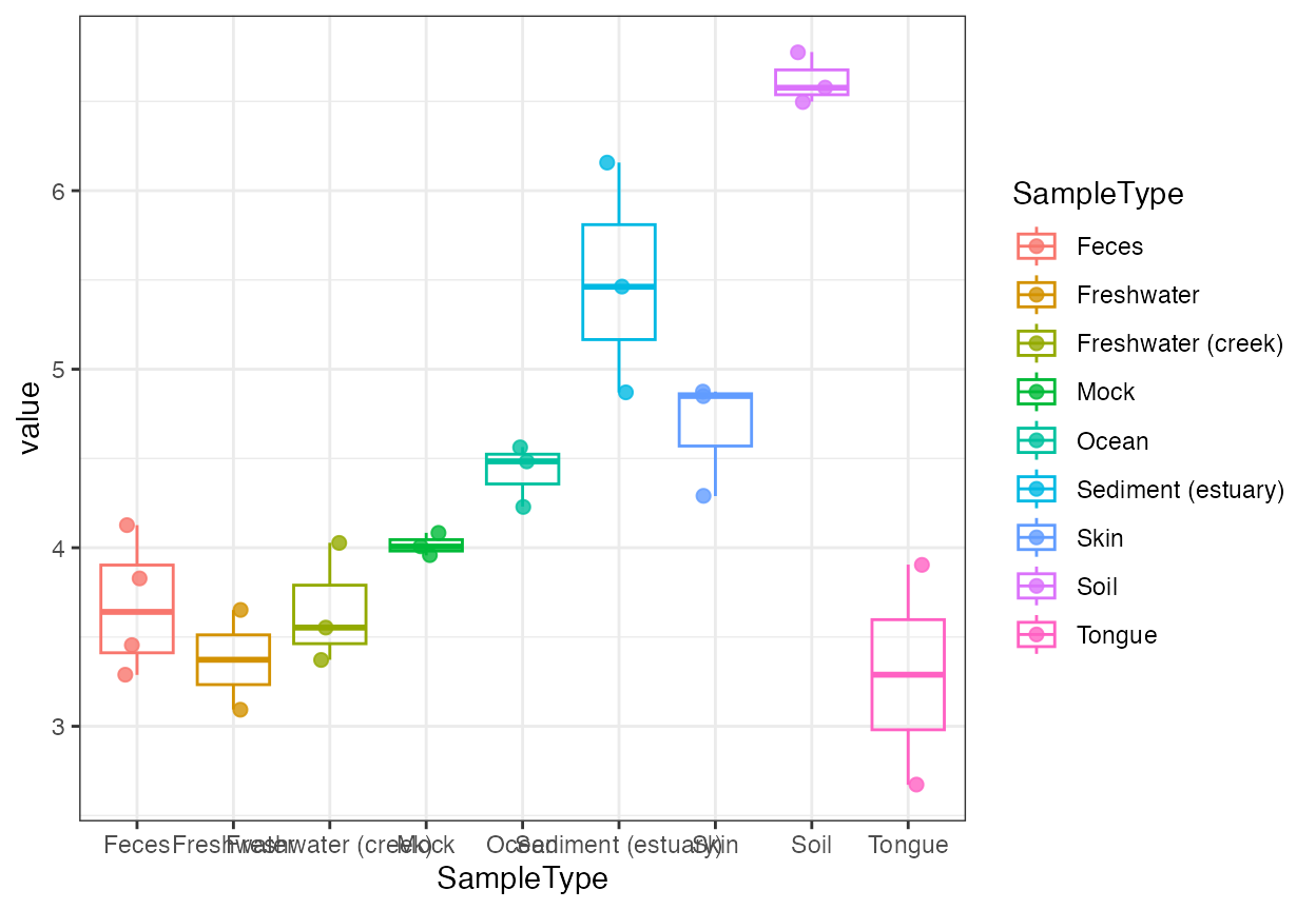
object <- global_patternsAlpha diversity
alpha <- calculate_alpha_diversity(object, metric = "shannon")
alpha
#> microbiome_diversity
#> Type: alpha
#> Method: shannon
#> Rows: 26

head(as_tibble_diversity(alpha))
#> # A tibble: 6 × 9
#>   sample_id value Primer  Final_Barcode Barcode_truncated_plus_T
#>   <chr>     <dbl> <fct>   <fct>         <fct>
#> 1 CL3        6.58 ILBC_01 AACGCA        TGCGTT
#> 2 CC1        6.78 ILBC_02 AACTCG        CGAGTT
#> 3 SV1        6.50 ILBC_03 AACTGT        ACAGTT
#> 4 M31Fcsw    3.83 ILBC_04 AAGAGA        TCTCTT
#> 5 M11Fcsw    3.29 ILBC_05 AAGCTG        CAGCTT
#> 6 M31Plmr    4.29 ILBC_07 AATCGT        ACGATT
#> # ℹ 4 more variables: Barcode_full_length <fct>, SampleType <fct>,
#> #   Description <fct>, class <chr>
plot_alpha_diversity(
  alpha,
  x = "SampleType",
  color_by = "SampleType"
)
Beta diversity
beta <- calculate_beta_diversity(object, method = "bray")
beta
#> microbiome_diversity
#> Type: beta
#> Method: bray
#> Samples: 26

dim(as.matrix(extract_diversity_result(beta)))
#> [1] 26 26
annotation <- stats::setNames(
  as.character(object@sample_info$SampleType),
  object@sample_info$sample_id
)

plot_beta_diversity(beta, annotate_by = annotation, cluster = TRUE)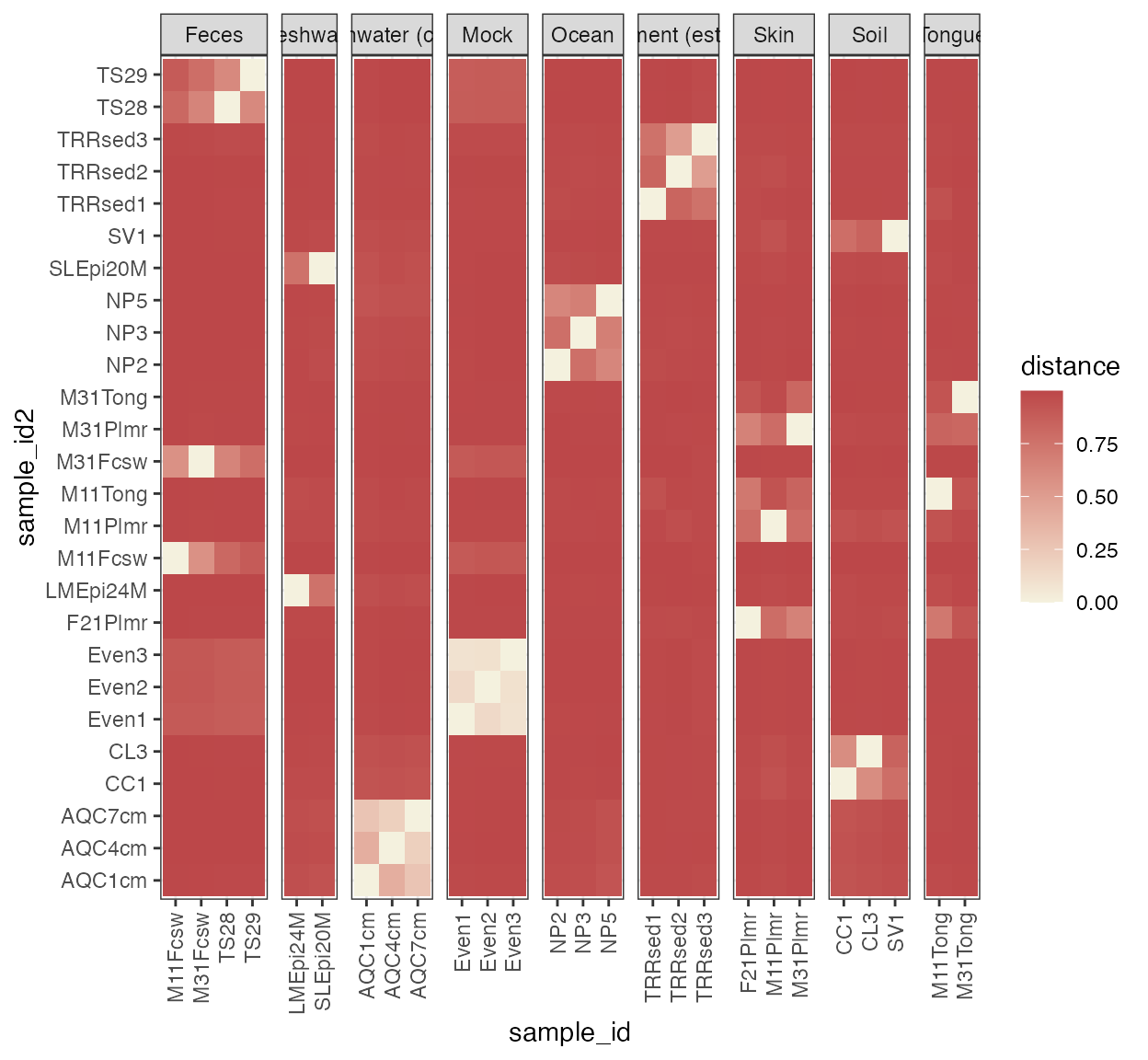
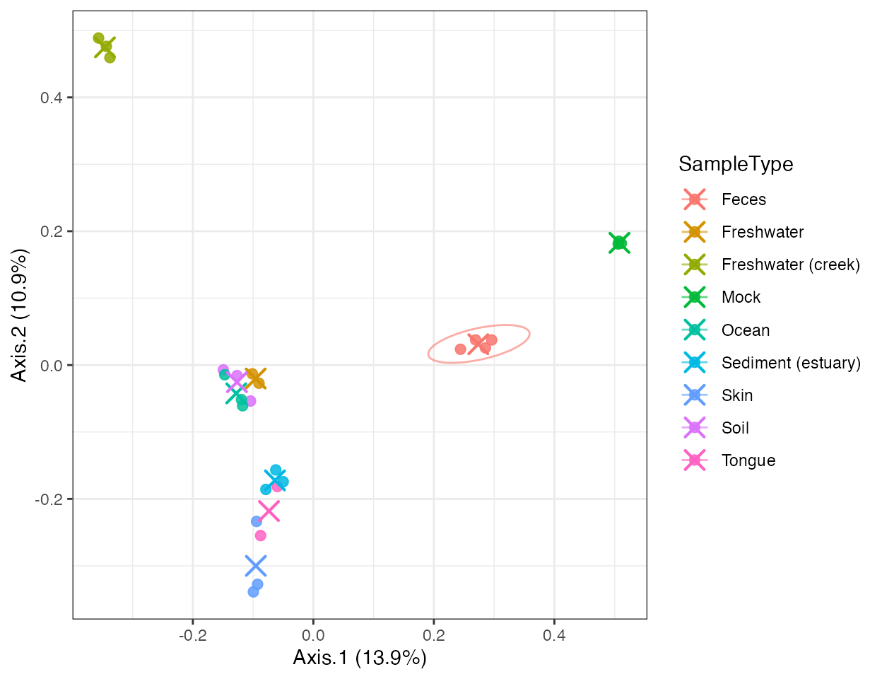
Ordination
pcoa <- run_ordination(object, method = "PCoA", distance_method = "bray")
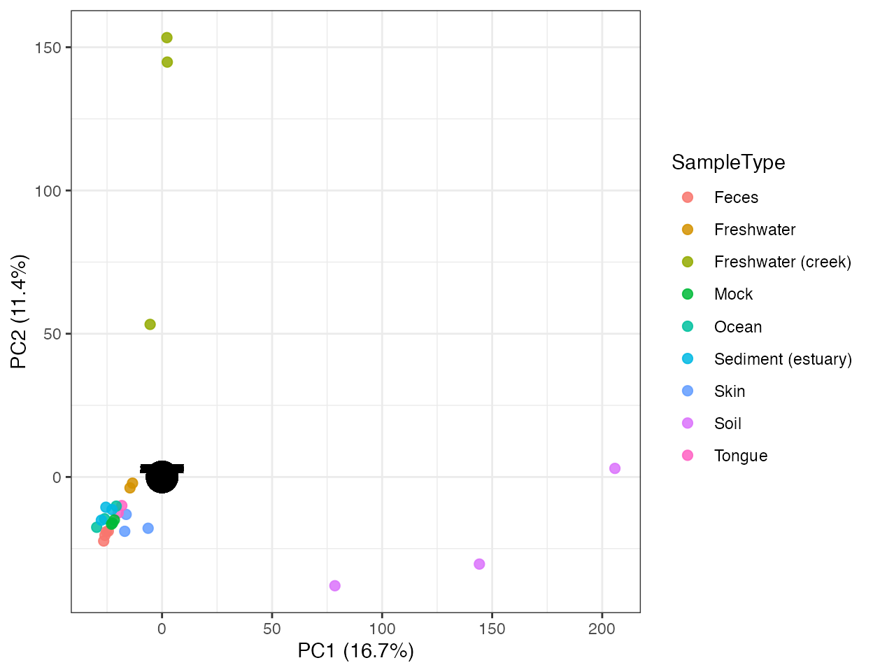
pca <- run_ordination(object, method = "PCA")
head(as_tibble_ordination(pcoa))
#> # A tibble: 6 × 10
#> Axis.1 Axis.2 sample_id Primer Final_Barcode Barcode_truncated_plus_T
#> <dbl> <dbl> <chr> <fct> <fct> <fct>
#> 1 -0.127 -0.0157 CL3 ILBC_01 AACGCA TGCGTT
#> 2 -0.149 -0.00714 CC1 ILBC_02 AACTCG CGAGTT
#> 3 -0.104 -0.0537 SV1 ILBC_03 AACTGT ACAGTT
#> 4 0.285 0.0258 M31Fcsw ILBC_04 AAGAGA TCTCTT
#> 5 0.244 0.0236 M11Fcsw ILBC_05 AAGCTG CAGCTT
#> 6 -0.0926 -0.328 M31Plmr ILBC_07 AATCGT ACGATT
#> # ℹ 4 more variables: Barcode_full_length <fct>, SampleType <fct>,
#> # Description <fct>, class <chr>
plot_ordination(
  pcoa,
  color_by = "SampleType",
  ellipse_by = "SampleType",
  centroid_by = "SampleType"
)
plot_ordination(
  pca,
  color_by = "SampleType",
  show_loading = TRUE,
  loading_scale = 2
)
Extract result tables
ordination_scores <- extract_ordination_result(pcoa)
diversity_values <- extract_diversity_result(alpha)

head(ordination_scores)
#>        Axis.1       Axis.2 sample_id  Primer Final_Barcode
#> 1 -0.12667533 -0.015709044       CL3 ILBC_01        AACGCA
#> 2 -0.14940705 -0.007137804       CC1 ILBC_02        AACTCG
#> 3 -0.10429782 -0.053710244       SV1 ILBC_03        AACTGT
#> 4  0.28543181  0.025755609   M31Fcsw ILBC_04        AAGAGA
#> 5  0.24415649  0.023606010   M11Fcsw ILBC_05        AAGCTG
#> 6 -0.09259285 -0.327628427   M31Plmr ILBC_07        AATCGT
#>   Barcode_truncated_plus_T Barcode_full_length SampleType
#> 1                   TGCGTT         CTAGCGTGCGT       Soil
#> 2                   CGAGTT         CATCGACGAGT       Soil
#> 3                   ACAGTT         GTACGCACAGT       Soil
#> 4                   TCTCTT         TCGACATCTCT      Feces
#> 5                   CAGCTT         CGACTGCAGCT      Feces
#> 6                   ACGATT         CGAGTCACGAT       Skin
#>                                  Description   class
#> 1   Calhoun South Carolina Pine soil, pH 4.9 Subject
#> 2   Cedar Creek Minnesota, grassland, pH 6.1 Subject
#> 3 Sevilleta new Mexico, desert scrub, pH 8.3 Subject
#> 4    M3, Day 1, fecal swab, whole body study Subject
#> 5   M1, Day 1, fecal swab, whole body study  Subject
#> 6    M3, Day 1, right palm, whole body study Subject
head(diversity_values)
#>   sample_id    value  Primer Final_Barcode Barcode_truncated_plus_T
#> 1       CL3 6.576517 ILBC_01        AACGCA                   TGCGTT
#> 2       CC1 6.776603 ILBC_02        AACTCG                   CGAGTT
#> 3       SV1 6.498494 ILBC_03        AACTGT                   ACAGTT
#> 4   M31Fcsw 3.828368 ILBC_04        AAGAGA                   TCTCTT
#> 5   M11Fcsw 3.287666 ILBC_05        AAGCTG                   CAGCTT
#> 6   M31Plmr 4.289269 ILBC_07        AATCGT                   ACGATT
#>   Barcode_full_length SampleType                                Description
#> 1         CTAGCGTGCGT       Soil   Calhoun South Carolina Pine soil, pH 4.9
#> 2         CATCGACGAGT       Soil   Cedar Creek Minnesota, grassland, pH 6.1
#> 3         GTACGCACAGT       Soil Sevilleta new Mexico, desert scrub, pH 8.3
#> 4         TCGACATCTCT      Feces    M3, Day 1, fecal swab, whole body study
#> 5         CGACTGCAGCT      Feces   M1, Day 1, fecal swab, whole body study
#> 6         CGAGTCACGAT       Skin    M3, Day 1, right palm, whole body study
#>     class
#> 1 Subject
#> 2 Subject
#> 3 Subject
#> 4 Subject
#> 5 Subject
#> 6 Subject