Advanced Visualization
Xiaotao Shen xiaotao.shen@outlook.com
2026-03-04
Source:vignettes/advanced_visualization.Rmd
advanced_visualization.RmdThis article focuses on heavier visualization layers that go beyond the core overview plots: interactive trees, pathway enrichment summaries, and standardized longitudinal mixed-effect result plots.
library(microbiomedataset)

data("global_patterns", package = "microbiomedataset")
data("demo_crossomics", package = "microbiomedataset")

tree_object <- align_tree(global_patterns, tree = "taxa_tree")
microbiome_object <- demo_crossomics$microbiome_data
metabolome_object <- demo_crossomics$metabolome_data
sample_link <- demo_crossomics$sample_link
Interactive tree panels
plot_tree_abundance(
  tree_object,
  tree = "taxa_tree",
  taxonomic_rank = "Phylum"
)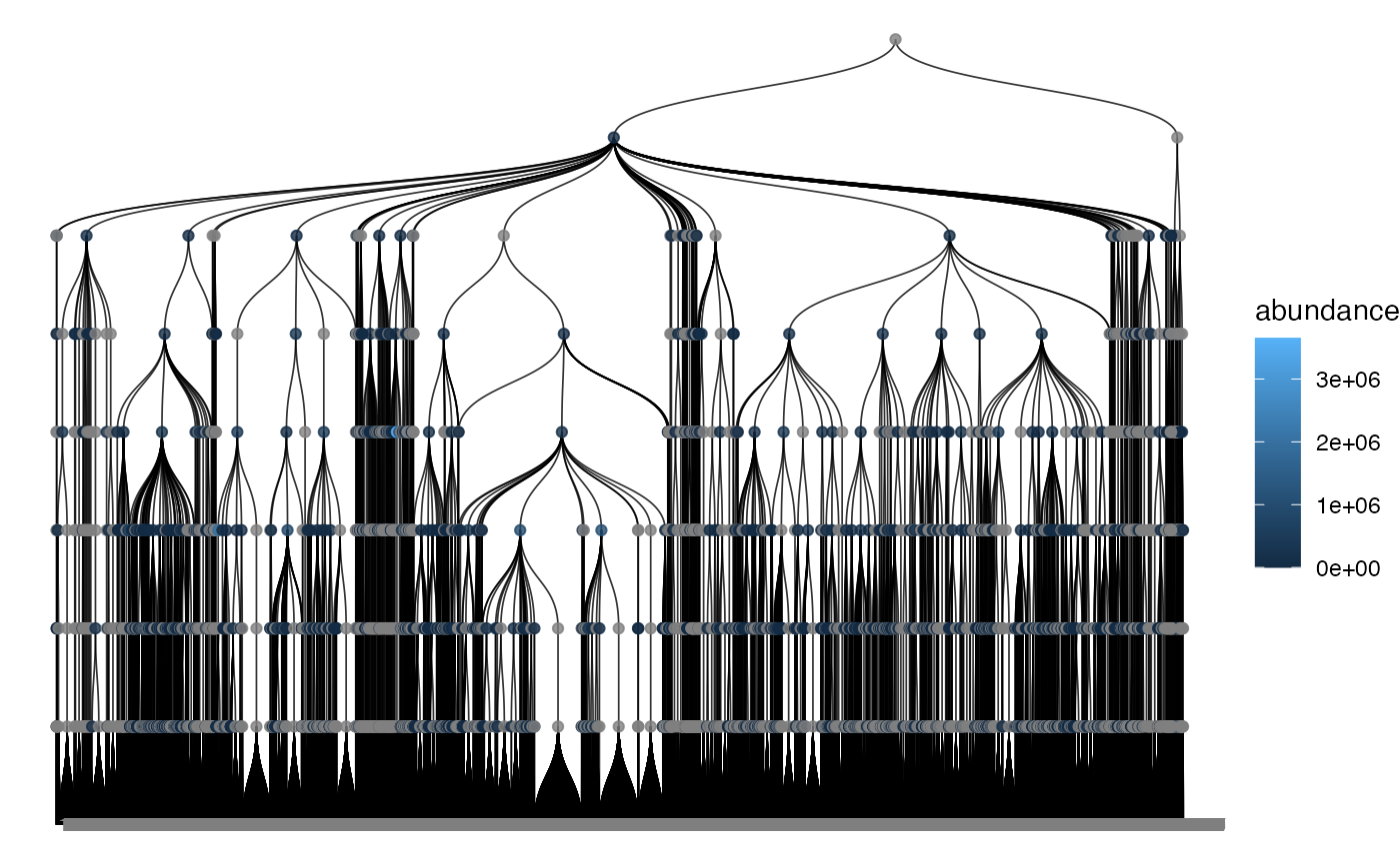
plot_tree_interactive(
  tree_object,
  tree = "taxa_tree",
  taxonomic_rank = "Phylum"
)
Pathway enrichment
association <- calculate_correlation(
  microbiome_data = microbiome_object,
  metabolome_data = metabolome_object,
  sample_link = sample_link,
  microbiome_rank = "Genus",
  metabolome_transform = "none"
)
pathway_link <- standardize_pathway_link(
  data.frame(
    taxon_id = summarise_taxa(
      microbiome_object,
      taxonomic_rank = "Genus"
    )@variable_info$variable_id[1],
    metabolite_id = metabolome_object@annotation_table$variable_id[1],
    pathway_id = "pathway_a",
    pathway_name = "Pathway A",
    stringsAsFactors = FALSE
  )
)
mechanism <- infer_metabolic_link(
  microbiome_data = microbiome_object,
  metabolome_data = metabolome_object,
  sample_link = sample_link,
  pathway_link = pathway_link,
  association_result = association,
  microbiome_rank = "Genus",
  q_value_cutoff = 1
)
enrichment_tbl <- calculate_pathway_enrichment(mechanism)
enrichment_tbl
#> # A tibble: 1 × 7
#>   pathway_id pathway_name n_background n_observed p_value q_value
#>   <chr>      <chr>               <int>      <int>   <dbl>   <dbl>
#> 1 pathway_a  Pathway A               1          1       1       1
#> # ℹ 1 more variable: enrichment_ratio <dbl>
plot_pathway_enrichment(mechanism)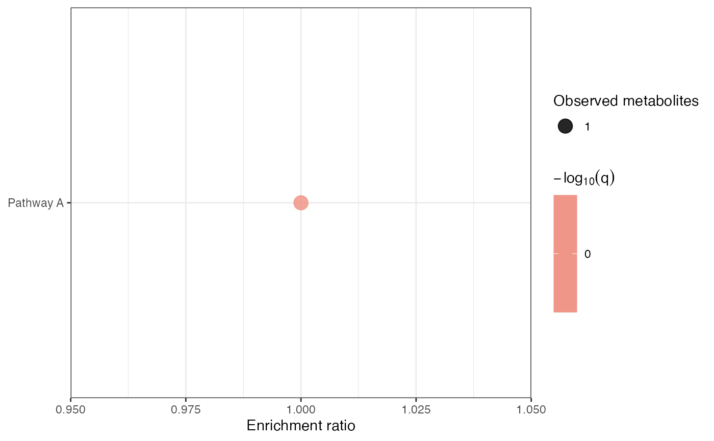
Longitudinal mixed-effect result plots
mixed_effect_result <- create_longitudinal_mixed_effect_result(
  result = data.frame(
    feature = paste0("Taxon_", 1:12),
    term = rep(c("age", "study_groupcontrol"), each = 6),
    estimate = c(seq(-0.5, 0.6, length.out = 6), seq(0.4, -0.4, length.out = 6)),
    lower_ci = c(seq(-0.7, 0.4, length.out = 6), seq(0.2, -0.6, length.out = 6)),
    upper_ci = c(seq(-0.3, 0.8, length.out = 6), seq(0.6, -0.2, length.out = 6)),
    p_value = seq(0.001, 0.12, length.out = 12),
    stringsAsFactors = FALSE
  ),
  method = "external_demo",
  time_variable = "age",
  group_variable = "study_group"
)
mixed_effect_result
#> longitudinal_mixed_effect_result
#> Method: external_demo
#> Time variable: age
#> Group variable: study_group
#> Rows: 12
plot_longitudinal_mixed_effect(mixed_effect_result, top_n = 10)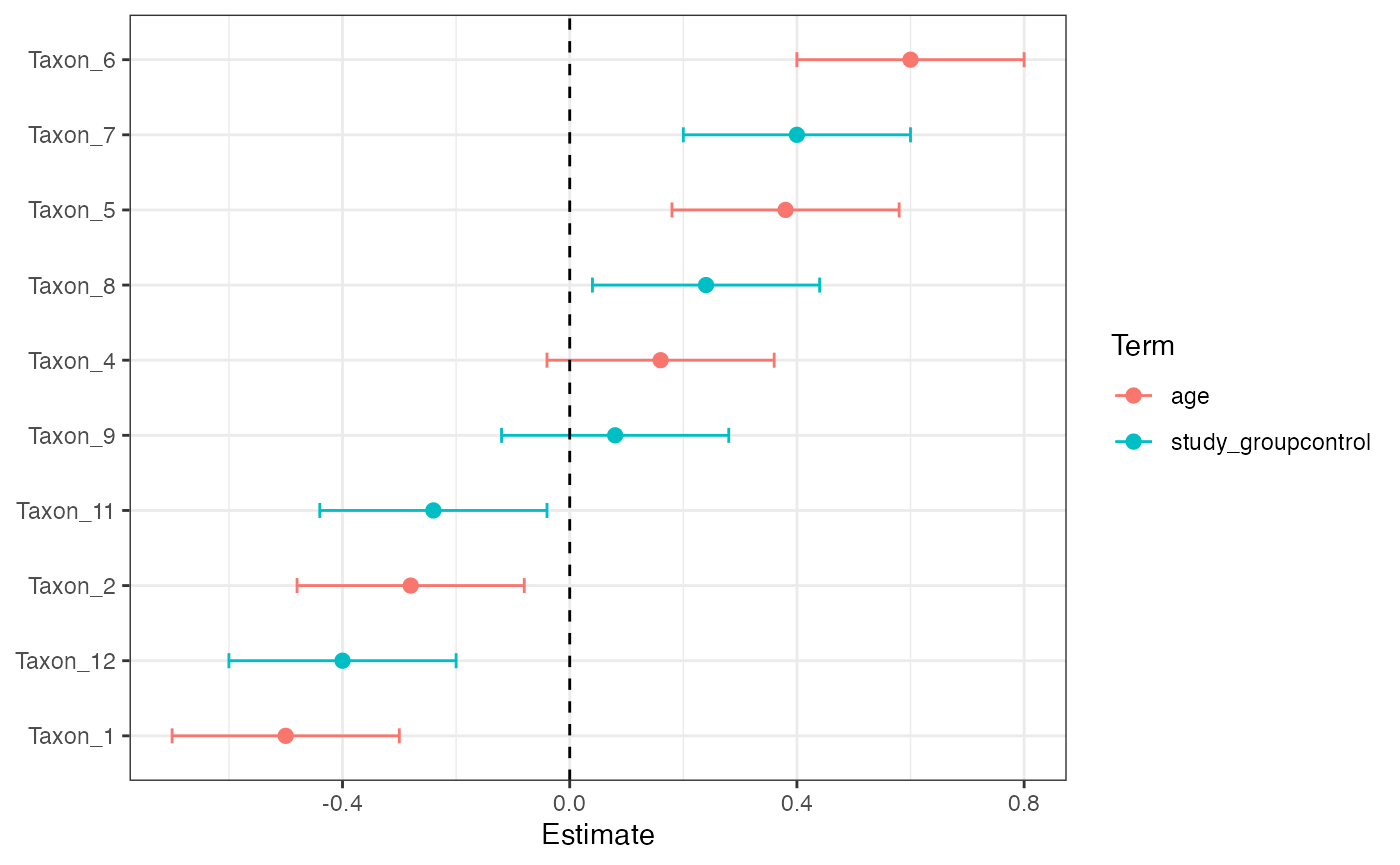
plot_longitudinal_effect_heatmap(mixed_effect_result, top_n = 10)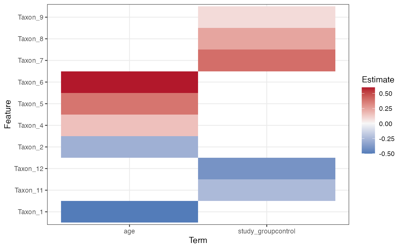
These advanced layers are designed to stay compatible with the same object system used elsewhere in the package, while still allowing external modeling results to be standardized into common plotting entry points.