Microbiome-metabolome integration

This article shows the first joint-analysis layer between microbiomedataset and massdataset using the packaged paired demo demo_crossomics. The demo was derived from the SINHA_CRC_2016 study in the Borenstein curated microbiome-metabolome collection and keeps a lightweight subset of paired samples, genera, and annotated metabolites.

library(microbiomedataset)
library(massdataset)

data("demo_crossomics", package = "microbiomedataset")

microbiome_object <- demo_crossomics$microbiome_data
metabolome_object <- demo_crossomics$metabolome_data
sample_link <- demo_crossomics$sample_link

demo_crossomics$selection
#> $study_id
#> [1] "SINHA_CRC_2016"
#> 
#> $sample_n
#> [1] 40
#> 
#> $taxon_n
#> [1] 60
#> 
#> $metabolite_n
#> [1] 48
#> 
#> $sample_rule
#> [1] "First 20 samples from each Study.Group after sorting by sample id."
#> 
#> $taxon_rule
#> [1] "Top genera by mean relative abundance among selected samples."
#> 
#> $metabolite_rule
#> [1] "Top high-confidence annotated metabolites by standard deviation, excluding X_-prefixed unknowns."

1. Start directly from microbiome and metabolome objects

aligned <- align_samples_between_omics(
  microbiome_data = microbiome_object,
  metabolome_data = metabolome_object,
  sample_link = sample_link
)

str(aligned, max.level = 1)
#> List of 3
#>  $ microbiome_data:Formal class 'microbiome_dataset' [package "microbiomedataset"] with 16 slots
#>  $ metabolome_data:Formal class 'mass_dataset' [package "massdataset"] with 11 slots
#>  $ sample_link    :'data.frame': 40 obs. of  3 variables:

The main API now starts from two native objects. Internally the package still knows how to build a paired object, but users do not need to create one first.

aligned$sample_link
#>    microbiome_sample_id metabolome_sample_id pair_id
#> 1               CRC.100              CRC.100 CRC.100
#> 2               CRC.102              CRC.102 CRC.102
#> 3               CRC.109              CRC.109 CRC.109
#> 4               CRC.110              CRC.110 CRC.110
#> 5               CRC.113              CRC.113 CRC.113
#> 6               CRC.116              CRC.116 CRC.116
#> 7                CRC.12               CRC.12  CRC.12
#> 8               CRC.132              CRC.132 CRC.132
#> 9               CRC.134              CRC.134 CRC.134
#> 10              CRC.135              CRC.135 CRC.135
#> 11              CRC.136              CRC.136 CRC.136
#> 12              CRC.139              CRC.139 CRC.139
#> 13              CRC.140              CRC.140 CRC.140
#> 14              CRC.141              CRC.141 CRC.141
#> 15              CRC.143              CRC.143 CRC.143
#> 16              CRC.146              CRC.146 CRC.146
#> 17              CRC.151              CRC.151 CRC.151
#> 18              CRC.156              CRC.156 CRC.156
#> 19              CRC.157              CRC.157 CRC.157
#> 20              CRC.160              CRC.160 CRC.160
#> 21               CRC.10               CRC.10  CRC.10
#> 22              CRC.104              CRC.104 CRC.104
#> 23              CRC.105              CRC.105 CRC.105
#> 24              CRC.118              CRC.118 CRC.118
#> 25              CRC.119              CRC.119 CRC.119
#> 26              CRC.121              CRC.121 CRC.121
#> 27              CRC.130              CRC.130 CRC.130
#> 28              CRC.144              CRC.144 CRC.144
#> 29              CRC.145              CRC.145 CRC.145
#> 30              CRC.149              CRC.149 CRC.149
#> 31              CRC.152              CRC.152 CRC.152
#> 32              CRC.161              CRC.161 CRC.161
#> 33              CRC.169              CRC.169 CRC.169
#> 34               CRC.17               CRC.17  CRC.17
#> 35              CRC.170              CRC.170 CRC.170
#> 36              CRC.171              CRC.171 CRC.171
#> 37              CRC.175              CRC.175 CRC.175
#> 38              CRC.180              CRC.180 CRC.180
#> 39              CRC.182              CRC.182 CRC.182
#> 40               CRC.19               CRC.19  CRC.19

2. Extract matched microbiome and metabolome matrices

matched <- extract_crossomics_matrix(
  microbiome_data = microbiome_object,
  metabolome_data = metabolome_object,
  sample_link = sample_link,
  microbiome_rank = "Genus",
  microbiome_transform = "relative",
  metabolome_transform = "none"
)

dim(matched$microbiome_matrix)
#> [1] 60 40
dim(matched$metabolome_matrix)
#> [1] 48 40
head(matched$sample_info[, c("pair_id", "microbiome_sample_id", "metabolome_sample_id")])
#>   pair_id microbiome_sample_id metabolome_sample_id
#> 1 CRC.100              CRC.100              CRC.100
#> 2 CRC.102              CRC.102              CRC.102
#> 3 CRC.109              CRC.109              CRC.109
#> 4 CRC.110              CRC.110              CRC.110
#> 5 CRC.113              CRC.113              CRC.113
#> 6 CRC.116              CRC.116              CRC.116

3. Export tidy long tables for joint plotting or modeling

long_tables <- melt_crossomics_features(
  microbiome_data = microbiome_object,
  metabolome_data = metabolome_object,
  sample_link = sample_link,
  microbiome_rank = "Genus"
)

head(long_tables$microbiome[, c("pair_id", "taxon_id", "abundance")])
#> # A tibble: 6 × 3
#>   pair_id taxon_id  abundance
#>   <chr>   <chr>         <dbl>
#> 1 CRC.100 Blautia_A    0.192 
#> 2 CRC.102 Blautia_A    0.0535
#> 3 CRC.109 Blautia_A    0.194 
#> 4 CRC.110 Blautia_A    0.115 
#> 5 CRC.113 Blautia_A    0.0388
#> 6 CRC.116 Blautia_A    0.0853
head(long_tables$metabolome[, c("pair_id", "metabolite_id", "abundance")])
#> # A tibble: 6 × 3
#>   pair_id metabolite_id abundance
#>   <chr>   <chr>             <dbl>
#> 1 CRC.100 CADAVERINE         4.44
#> 2 CRC.102 CADAVERINE        -1.43
#> 3 CRC.109 CADAVERINE        -1.39
#> 4 CRC.110 CADAVERINE        -1.82
#> 5 CRC.113 CADAVERINE         2.35
#> 6 CRC.116 CADAVERINE        -4.49

4. Compute taxon-metabolite associations

association <- associate_microbe_metabolite(
  microbiome_data = microbiome_object,
  metabolome_data = metabolome_object,
  sample_link = sample_link,
  microbiome_rank = "Genus",
  metabolome_transform = "none",
  method = "spearman"
)

association
#> microbe_metabolite_association
#> Method: spearman
#> Microbiome rank: Genus
#> Rows: 2880
head(association@result[, c("taxon_id", "metabolite_id", "estimate", "q_value")])
#>    taxon_id      metabolite_id    estimate   q_value
#> 1 Blautia_A         CADAVERINE  0.07958667 0.9442916
#> 2 Blautia_A  _1_METHYLXANTHINE  0.44323514 0.5576252
#> 3 Blautia_A             DHEA_S  0.11069418 0.9377717
#> 4 Blautia_A       GLYCOCHOLATE  0.15214231 0.9252912
#> 5 Blautia_A           PIPERINE  0.10520883 0.9405171
#> 6 Blautia_A _4_ACETAMIDOPHENOL -0.11765810 0.9309772

5. Build a correlation network

correlation <- calculate_correlation(
  microbiome_data = microbiome_object,
  metabolome_data = metabolome_object,
  sample_link = sample_link,
  microbiome_rank = "Genus",
  metabolome_transform = "none",
  method = "spearman"
)

correlation_network <- build_correlation_network(
  correlation,
  min_abs_correlation = 0.2,
  max_q_value = 1,
  top_n = 20
)

correlation_network
#> microbe_metabolite_network
#> Method: spearman
#> Microbiome rank: Genus
#> Nodes: 32
#> Edges: 20
head(extract_network_table(correlation_network)$edges)
#>                 from                    to     weight   q_value direction
#> 1 Pseudobutyrivibrio _1_3_7_TRIMETHYLURATE -0.5574928 0.4263273  negative
#> 2     Clostridioides               CITRATE -0.5324578 0.4263273  negative
#> 3       Ruminococcus          SACCHAROPINE  0.5274169 0.4263273  positive
#> 4         Klebsiella         GALACTURONATE  0.5114404 0.4263273  positive
#> 5        Haemophilus   _5_HYDROXYHEXANOATE -0.5018603 0.4263273  negative
#> 6       Ruminococcus _1_3_7_TRIMETHYLURATE  0.4996248 0.4263273  positive
#>     method
#> 1 spearman
#> 2 spearman
#> 3 spearman
#> 4 spearman
#> 5 spearman
#> 6 spearman

plot_correlation_network(correlation_network)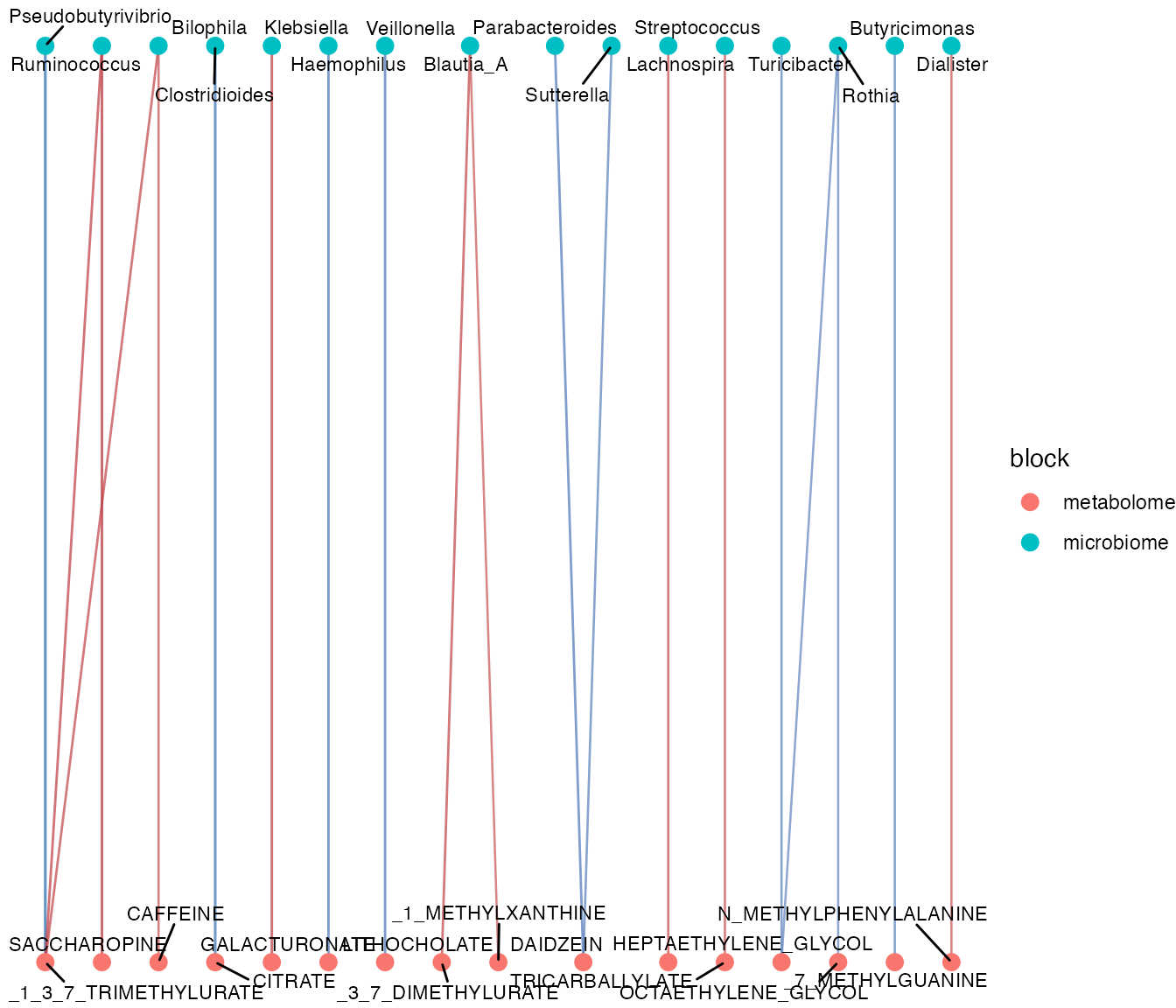

Bipartite network connecting microbiome taxa and metabolites using top correlation edges.

module_table <- detect_network_modules(correlation_network)
summarise_network_modules(module_table)
#> # A tibble: 12 × 4
#>    module n_nodes n_microbiome n_metabolome
#>     <int>   <int>        <int>        <int>
#>  1      1       6            3            3
#>  2      2       4            2            2
#>  3      3       3            1            2
#>  4      4       3            2            1
#>  5      5       2            1            1
#>  6      6       2            1            1
#>  7      7       2            1            1
#>  8      8       2            1            1
#>  9      9       2            1            1
#> 10     10       2            1            1
#> 11     11       2            1            1
#> 12     12       2            1            1

6. Add pathway metadata for mechanism-oriented evidence

genus_object <- summarise_taxa(microbiome_object, taxonomic_rank = "Genus")
pathway_link <- data.frame(
  taxon_id = genus_object@variable_info$variable_id[1],
  metabolite_id = metabolome_object@annotation_table$variable_id[
    which(!is.na(metabolome_object@annotation_table$kegg_id))[1]
  ],
  pathway_id = "example_kegg_pathway",
  pathway_name = "Example pathway",
  evidence_type = "annotation_overlap",
  stringsAsFactors = FALSE
)
pathway_link <- standardize_pathway_link(pathway_link)

mechanism <- infer_metabolic_link(
  microbiome_data = microbiome_object,
  metabolome_data = metabolome_object,
  sample_link = sample_link,
  pathway_link = pathway_link,
  microbiome_rank = "Genus",
  q_value_cutoff = 1
)

head(mechanism@result[, c("taxon_id", "metabolite_id", "pathway_id", "mechanism_score")])
#>           taxon_id      metabolite_id pathway_id mechanism_score
#> 1      Bacteroides    TRICARBALLYLATE       <NA>       0.5397279
#> 2        Blautia_A _3_7_DIMETHYLURATE       <NA>       0.3145413
#> 3 Faecalibacterium  TRYPTOPHYLPROLINE       <NA>       0.2941110
#> 4      Coprobacter         PUTRESCINE       <NA>       0.2847937
#> 5          Dorea_A  _1_METHYLXANTHINE       <NA>       0.2841477
#> 6       Prevotella  _1_METHYLXANTHINE       <NA>       0.2730807

taxon_pathway_link <- standardize_taxon_pathway_link(
  data.frame(
    taxon_id = pathway_link$taxon_id,
    pathway_id = pathway_link$pathway_id,
    pathway_name = "Lipid pathway"
  )
)

summarise_pathways(mechanism, taxon_pathway_link = taxon_pathway_link)
#> # A tibble: 1 × 6
#>   pathway_id           pathway_name    n_taxa n_metabolites mean_mechanism_score
#>   <chr>                <chr>            <int>         <int>                <dbl>
#> 1 example_kegg_pathway Example pathway      1             1              0.00100
#> # ℹ 1 more variable: max_mechanism_score <dbl>

7. Run latent integration

if (requireNamespace("mixOmics", quietly = TRUE)) {
  integration <- integrate_microbe_metabolite(
    microbiome_data = microbiome_object,
    metabolome_data = metabolome_object,
    sample_link = sample_link,
    microbiome_rank = NULL,
    method = "spls",
    ncomp = 2
  )
  
  integration
}
#> crossomics_integration
#> Method: spls
#> Microbiome rank: 
#> Components: 2
#> Samples: 40
#> Microbiome loadings: 60
#> Metabolome loadings: 48

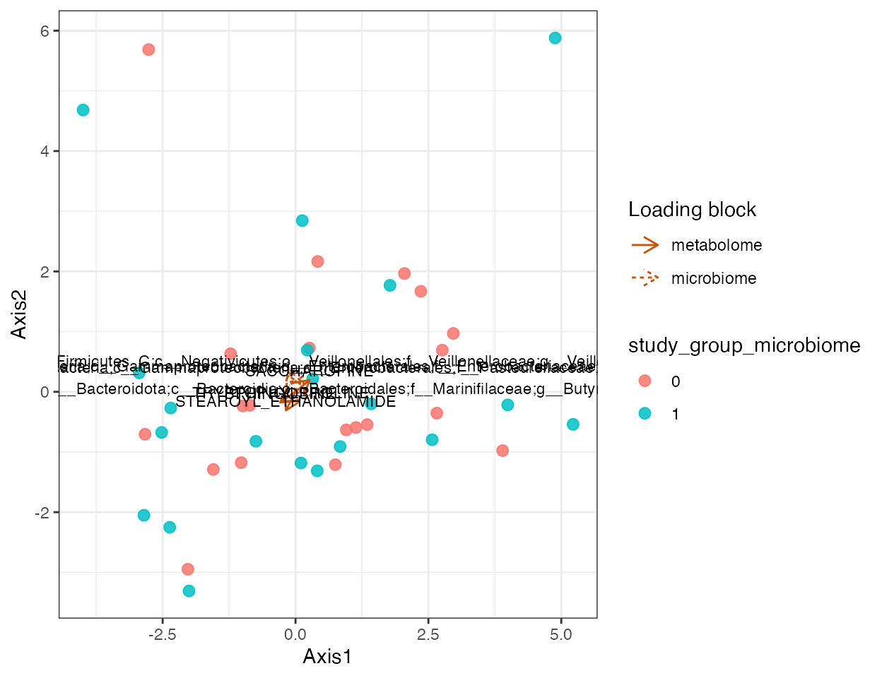
plot_crossomics_integration(
  integration,
  color_by = "study_group_microbiome",
  show_loading = TRUE,
  top_n = 4
)

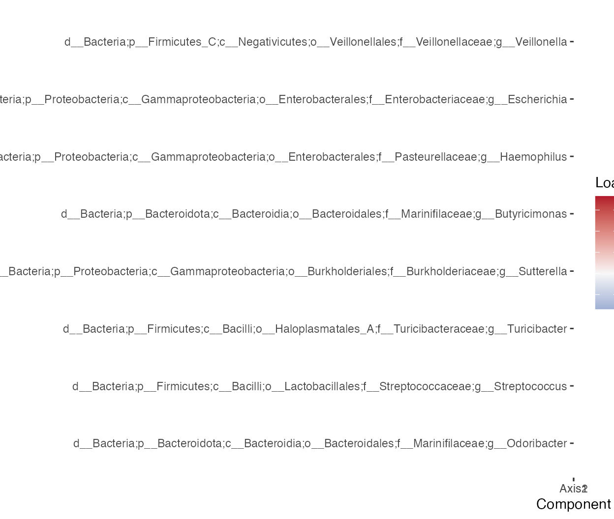
Cross-omics integration scatter plot with sample coordinates and top loading arrows from microbiome and metabolome blocks.

plot_crossomics_loading_heatmap(
  integration,
  block = "microbiome",
  top_n = 8
)

Heatmap of top microbiome loading features across latent integration components.

plot_crossomics_network(
  association,
  top_n = 12
)

Bipartite network connecting microbiome taxa and metabolites using top cross-omics association edges.

Summary

This first cross-omics layer is designed around three ideas:

keep microbiome and metabolome as native domain-specific objects;
use function-style joint analysis as the main user interface;
keep the paired joint object as an optional advanced container when persistent link metadata is useful.

Xiaotao Shen xiaotao.shen@outlook.com

2026-03-04