End-to-end microbiome workflow

This article shows a compact tutorial-style workflow built entirely on the package demo data.

library(microbiomedataset)
data("global_patterns", package = "microbiomedataset")

object <- global_patterns
object
#> -------------------- 
#> microbiomedataset version: 0.99.1 
#> -------------------- 
#> 1.expression_data:[ 19216 x 26 data.frame]
#> 2.sample_info:[ 26 x 8 data.frame]
#> 3.variable_info:[ 19216 x 8 data.frame]
#> 4.sample_info_note:[ 8 x 2 data.frame]
#> 5.variable_info_note:[ 8 x 2 data.frame]
#> -------------------- 
#> Processing information (extract_process_info())
#> create_microbiome_dataset ---------- 
#>             Package               Function.used                Time
#> 1 microbiomedataset create_microbiome_dataset() 2022-07-11 01:56:13

1. Prepare the dataset

Keep only samples with clear biological grouping and taxa with genus annotation.

object <-
  object %>%
  activate_microbiome_dataset("sample_info") %>%
  dplyr::filter(SampleType %in% c("Feces", "Skin", "Tongue", "Soil")) %>%
  activate_microbiome_dataset("variable_info") %>%
  dplyr::filter(!is.na(Genus))

dim(object@expression_data)
#> [1] 8008   12
table(object@sample_info$SampleType)
#> 
#>              Feces         Freshwater Freshwater (creek)               Mock 
#>                  4                  0                  0                  0 
#>              Ocean Sediment (estuary)               Skin               Soil 
#>                  0                  0                  3                  3 
#>             Tongue 
#>                  2

2. Aggregate and transform abundance

genus_relative <-
  transform_taxa(
    object,
    taxonomic_rank = "Genus",
    what = "sum_intensity",
    method = "relative"
  )

colSums(genus_relative@expression_data)[1:5]
#>     CL3     CC1     SV1 M31Fcsw M11Fcsw 
#>       1       1       1       1       1

Export a long table for downstream plotting or modeling:

genus_table <- melt_taxa(
  object,
  taxonomic_rank = "Genus",
  relative = TRUE
)

head(genus_table[, c("sample_id", "Genus", "abundance")])
#>   sample_id         Genus   abundance
#> 1       CC1          4-29 0.000641909
#> 2       CC1      4041AA30 0.000000000
#> 3       CC1           A17 0.907659258
#> 4       CC1   Abiotrophia 0.000000000
#> 5       CC1 Acaryochloris 0.000000000
#> 6       CC1   Acetivibrio 0.000000000

3. Quantify diversity

alpha <- calculate_alpha_diversity(object, metric = "shannon")
beta <- calculate_beta_diversity(object, method = "bray")

head(as_tibble_diversity(alpha))
#> # A tibble: 6 × 9
#>   sample_id value Primer  Final_Barcode Barcode_truncated_plus_T
#>   <chr>     <dbl> <fct>   <fct>         <fct>                   
#> 1 CL3        5.22 ILBC_01 AACGCA        TGCGTT                  
#> 2 CC1        5.22 ILBC_02 AACTCG        CGAGTT                  
#> 3 SV1        5.42 ILBC_03 AACTGT        ACAGTT                  
#> 4 M31Fcsw    3.21 ILBC_04 AAGAGA        TCTCTT                  
#> 5 M11Fcsw    2.69 ILBC_05 AAGCTG        CAGCTT                  
#> 6 M31Plmr    3.99 ILBC_07 AATCGT        ACGATT                  
#> # ℹ 4 more variables: Barcode_full_length <fct>, SampleType <fct>,
#> #   Description <fct>, class <chr>

plot_alpha_diversity(alpha, x = "SampleType", color_by = "SampleType")

Boxplot and jitter plot of Shannon alpha diversity grouped by sample type.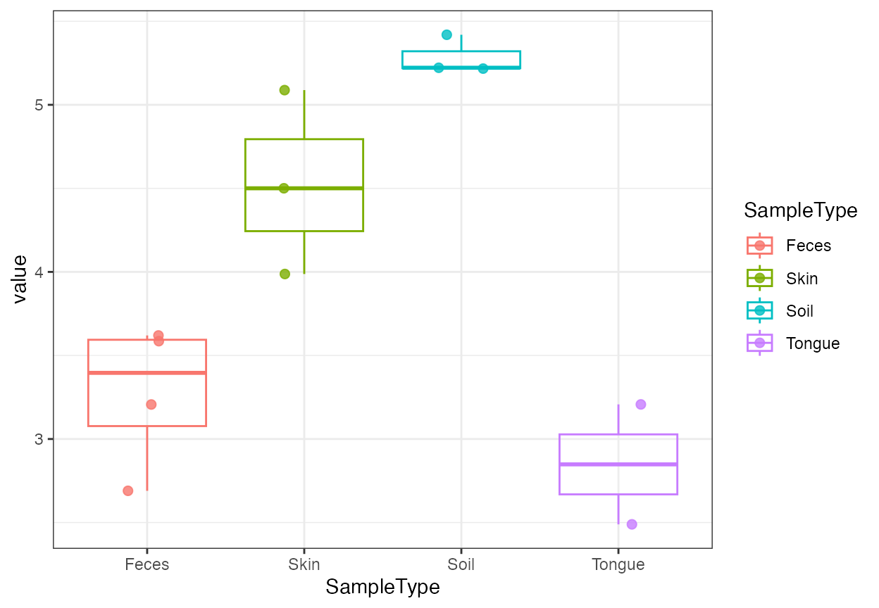

annotation <- stats::setNames(
  as.character(object@sample_info$SampleType),
  object@sample_info$sample_id
)
plot_beta_diversity(beta, annotate_by = annotation, cluster = TRUE)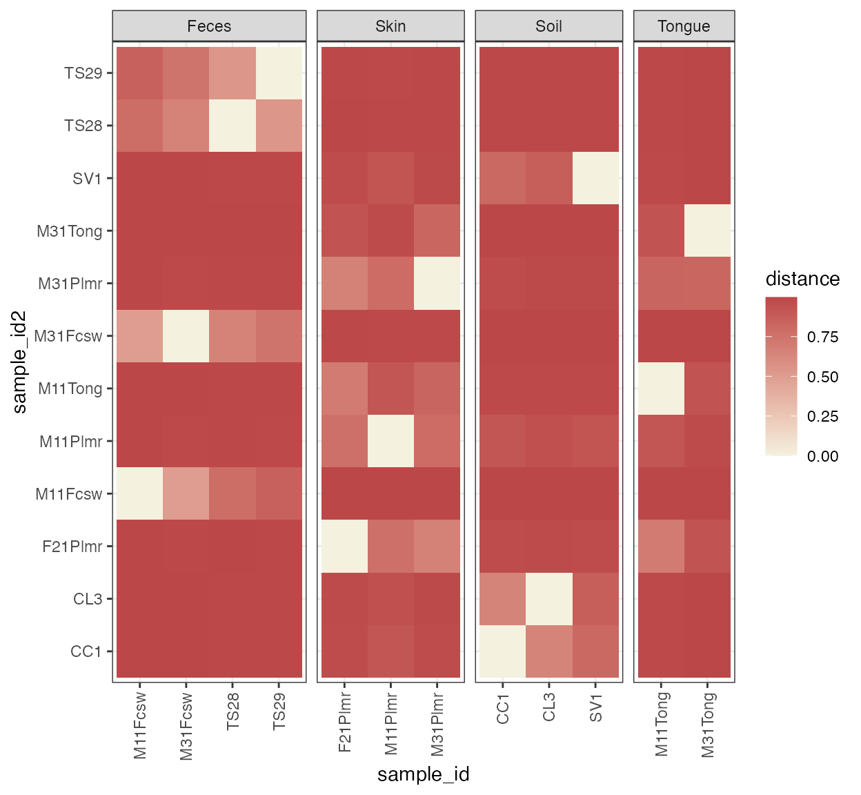

Heatmap of Bray-Curtis beta diversity distances with sample type annotations and clustered samples.

4. Run ordination

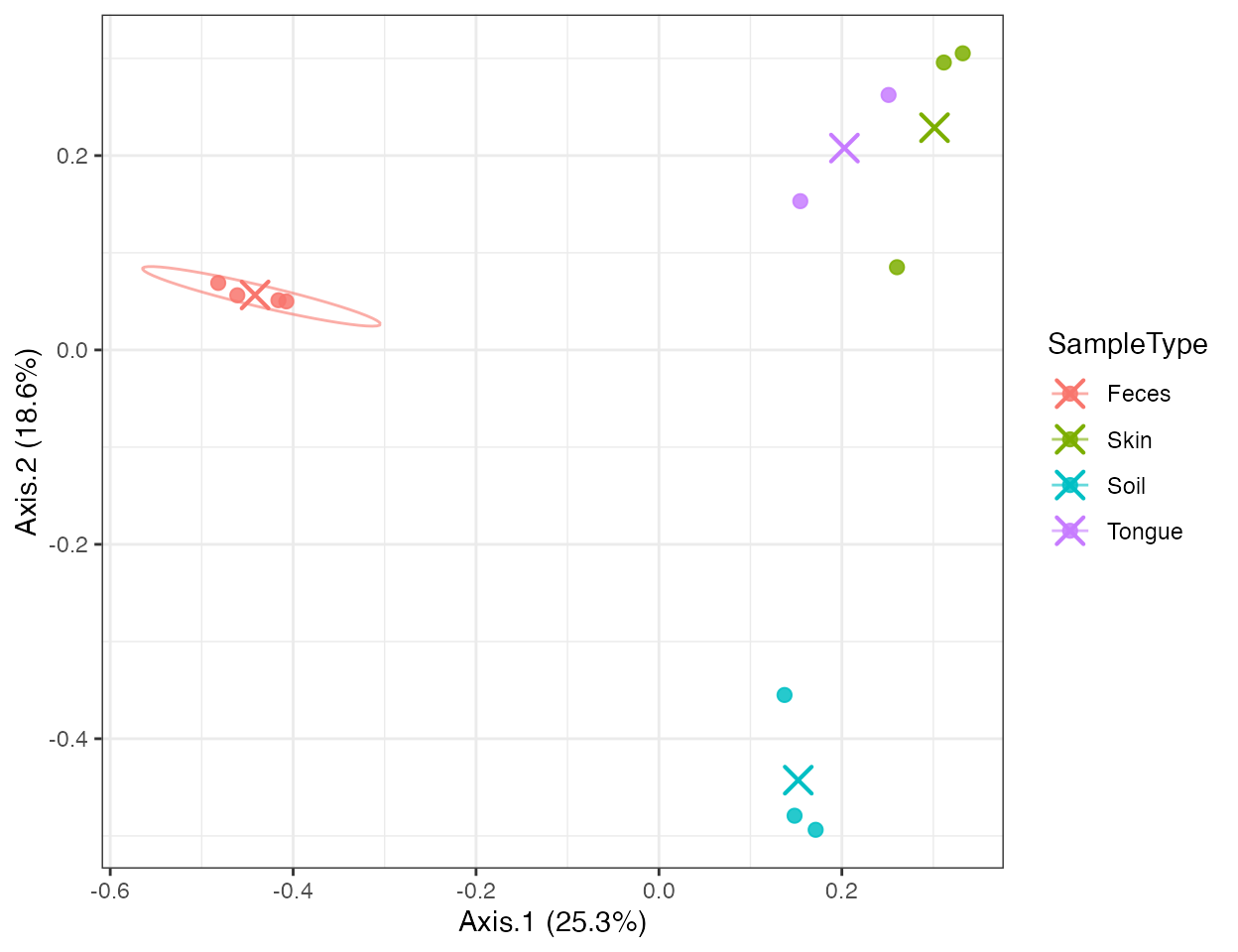
pcoa <- run_ordination(object, method = "PCoA", distance_method = "bray")
head(as_tibble_ordination(pcoa))
#> # A tibble: 6 × 10
#>   Axis.1  Axis.2 sample_id Primer  Final_Barcode Barcode_truncated_plus_T
#>    <dbl>   <dbl> <chr>     <fct>   <fct>         <fct>                   
#> 1  0.148 -0.479  CL3       ILBC_01 AACGCA        TGCGTT                  
#> 2  0.171 -0.494  CC1       ILBC_02 AACTCG        CGAGTT                  
#> 3  0.137 -0.355  SV1       ILBC_03 AACTGT        ACAGTT                  
#> 4 -0.482  0.0690 M31Fcsw   ILBC_04 AAGAGA        TCTCTT                  
#> 5 -0.416  0.0512 M11Fcsw   ILBC_05 AAGCTG        CAGCTT                  
#> 6  0.312  0.296  M31Plmr   ILBC_07 AATCGT        ACGATT                  
#> # ℹ 4 more variables: Barcode_full_length <fct>, SampleType <fct>,
#> #   Description <fct>, class <chr>

plot_ordination(
  pcoa,
  color_by = "SampleType",
  ellipse_by = "SampleType",
  centroid_by = "SampleType"
)

PCoA ordination scatter plot colored by sample type with ellipses and centroids.

5. Attach and visualize trees

tree_object <- convert2microbiome_dataset(convert2phyloseq(object))
melt_tree(tree_object, tree = "taxa_tree")[1:6, 1:5]
#>        tree parent node label   nodeClass
#> 1 taxa_tree   9486    1  5011 variable_id
#> 2 taxa_tree   9487    2  5009 variable_id
#> 3 taxa_tree   9488    3  5008 variable_id
#> 4 taxa_tree   9488    4  5010 variable_id
#> 5 taxa_tree   9489    5  5006 variable_id
#> 6 taxa_tree   9489    6  5007 variable_id

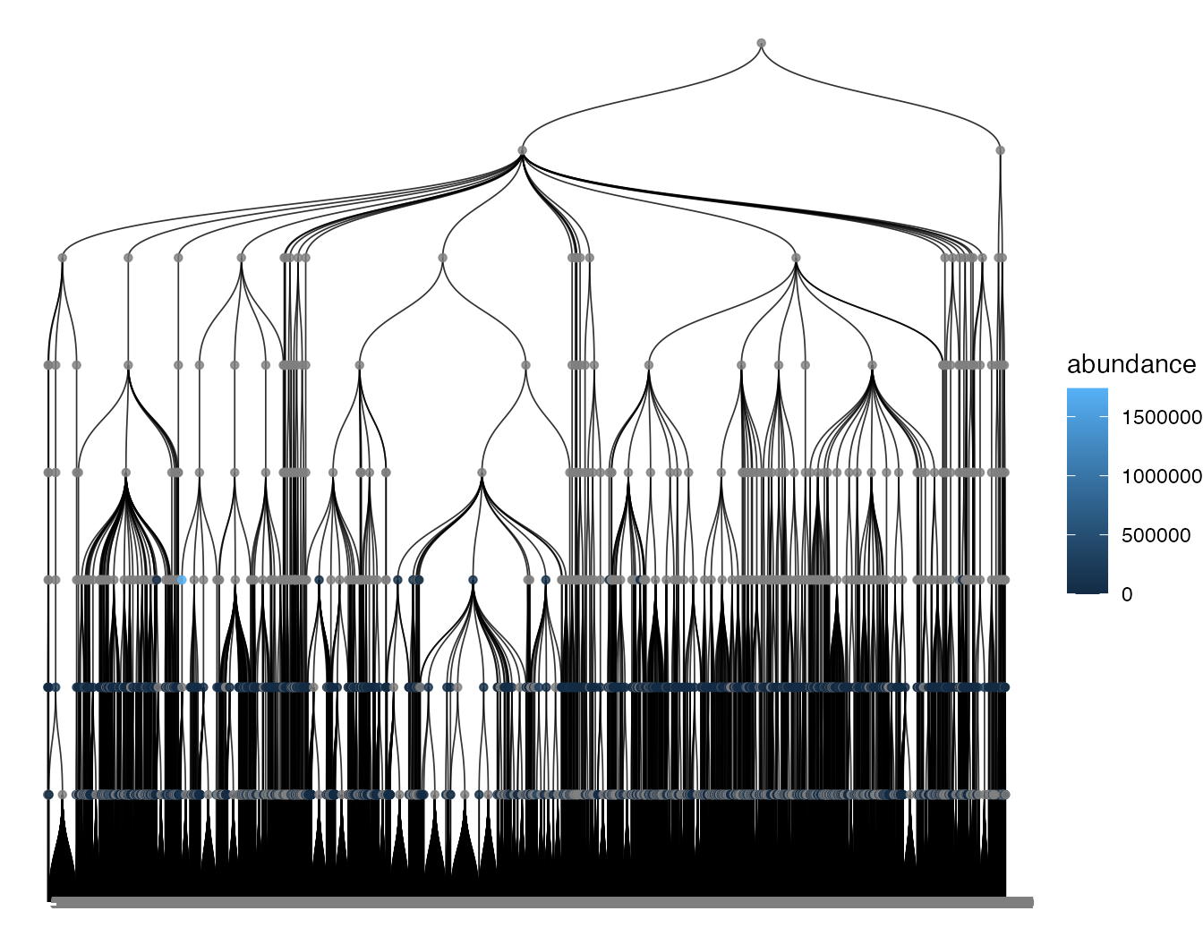
plot_tree(
  tree_object,
  tree = "taxa_tree",
  color_by = "abundance",
  taxonomic_rank = "Phylum"
)

Taxonomy tree plot with phylum-level abundance mapped to node color in the workflow example.

6. Export attachments for external tools

ref_seq <- Biostrings::DNAStringSet(rep("ACGT", nrow(tree_object@variable_info)))
tree_object <- replace_ref_seq(tree_object, value = ref_seq)

fasta_file <- tempfile(fileext = ".fasta")
tree_file <- tempfile(fileext = ".nwk")

export_ref_seq(tree_object, fasta_file)
export_tree(tree_object, tree_file, tree = "taxa_tree", format = "newick")

file.exists(fasta_file)
#> [1] TRUE
file.exists(tree_file)
#> [1] TRUE

Summary

This workflow shows the intended layering of microbiomedataset:

start with a synchronized microbiome object;
use tidy verbs and explicit microbiome verbs for filtering and aggregation;
compute diversity and ordination inside the same object ecosystem;
move trees and sequences in and out when needed.

Xiaotao Shen xiaotao.shen@outlook.com

2026-03-04